Estimating effect sizes with a DeepDive Model

This tutorial demonstrates how to estimate effect sizes with a DeepDive model on single-cell ATAC-seq data.

---

Imports

import scanpy as sc
import DeepDive
import seaborn as sns
import numpy as np
import matplotlib.pyplot as plt

from utils import reads_to_fragments

1. Load and preprocess the dataset

We start with an AnnData object containing single-cell chromatin accessibility profiles. Here we use the liver sciATAC-seq3 dataset (sciatac3_liver_10k.h5ad), subset from the full dataset (dataset and preprocessing better described in the training.ipynb notebook).

adata = sc.read_h5ad('data/sciatac3_liver_10k.h5ad')

# Filter genes detected in fewer than 1% of cells
min_cells = int(adata.shape[0] * 0.01)
sc.pp.filter_genes(adata, min_cells=min_cells)

# Ensure unique cell IDs
adata.obs_names_make_unique()

# Convert raw reads into fragments
reads_to_fragments(adata)
adata.X = adata.layers['fragments']

2. Define model and training parameters

We specify model hyperparameters and training settings.

n_decoders = 5
model_params = {
    'n_epochs_pretrain_ae' : 200*n_decoders,
    'n_decoders' : n_decoders,
}
train_params = {
    'max_epoch' : 300*n_decoders,
    'batch_size' : 1024,
    'shuffle' : True
}

discrete_covriate_keys = ['sample_name', 'sex', 'batch', 'cell_type']
continuous_covriate_keys = ['day_of_pregnancy']

3. Train DeepDive

We initialize and train the model using the training dataset.

model = DeepDive.DeepDive(adata = adata,
                        discrete_covariate_names = discrete_covriate_keys,
                        continuous_covariate_names = continuous_covriate_keys,
                        **model_params
                       )

model.train_model(adata, None,
                  **train_params)

Epoch Train [1500 / 1500]: 100%|██████████| 10/10 [00:00<00:00, 10.10it/s, ETA=01d:00h:21:m41s|01d:00h:21:m41s, kl_loss=1.68, recon_loss=3.15e+3]

4. Compare groups

The DeepDive.compare_groups() function identifies accessible regions that differ between two groups independent of disentangled covariates.

In this example, we compare Hepatoblasts and Erythroblasts to identify differential chromatin accessibility patterns.

da = DeepDive.compare_groups(model, adata, 'cell_type', groupA = 'Hepatoblasts', groupB = 'Erythroblasts')

da.head()

	Feature	groupA	groupB	Difference	Zscore	Pvalue	FDR
0	chr1:565561-565842	0.808578	-1.587507	2.396085	1.704382	0.006697	0.055971
1	chr1:569259-569557	2.841677	1.127797	1.713880	1.223938	0.128054	0.535595
2	chr1:569659-569951	1.822991	-0.457494	2.280485	1.626589	0.011054	0.082341
3	chr1:713647-714744	0.733735	0.902667	-0.168932	-0.094762	0.999939	1.000000
4	chr1:762075-763248	-0.183651	-0.042263	-0.141388	-0.077697	0.999797	1.000000

This returns a DataFrame containing:

• Difference: Effect size between the two groups

• FDR: False discovery rate (multiple testing–corrected p-value)

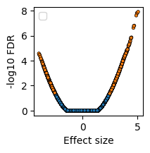
We can visualize the differential results as a volcano plot.

plt.subplots(figsize=(2,2))
sns.scatterplot(
    x=da.Difference,
    y=-np.log10(da.FDR),
    hue=da.FDR < 0.05,
    edgecolor='k',
    linewidth=0.5,
    s=10
)
plt.legend([])
plt.ylabel('-log10 FDR')
plt.xlabel('Effect size')

Text(0.5, 0, 'Effect size')

5. Compare groups with covariate constraints

DeepDive can also control for confounding factors by fixing certain covariates. For example, to compare Hepatoblasts vs Erythroblasts while holding sex = female constant:

background = {'sex':'female'}
da = DeepDive.compare_groups(model, adata, 'cell_type', groupA = 'Hepatoblasts', groupB = 'Erythroblasts', background = background)

This performs the same comparison as above but within the context of a fixed background covariate — allowing interpretation of group differences dependent the sex.

Summary

• DeepDive.compare_groups() quantifies differential effects between categorical groups.

• Supports covariate-controlled comparisons via the background argument.

• Returns a feature-level DataFrame with effect sizes and FDR-adjusted p-values.